Sequential analysis with a maximum of 3 looks (Fisher’s combination test design)
Full last stage level design, binding futility, one-sided overall significance level 2.5%, undefined endpoint.
Stage
1
2
3
Fixed weight
1
1
1
Cumulative alpha spent
0.0084
0.0128
0.0250
Stage levels (one-sided)
0.0084
0.0084
0.0250
Efficacy boundary (p product scale)
0.0084123
0.0010734
0.0007284
Futility boundary (separate p-value scale)
0.5000
1.0000
Problem
For group sequential designs, futility bounds have to be specified on the \(z\)-value scale. For Fisher’s combination test, they are on the separate \(p\)-value scale
It is desired, however, to define it also for other scales, e.g., the conditional power scale
On the effect size scale, futility bounds are already the output in the getSampleSize...() and getPower...() functions. For example:
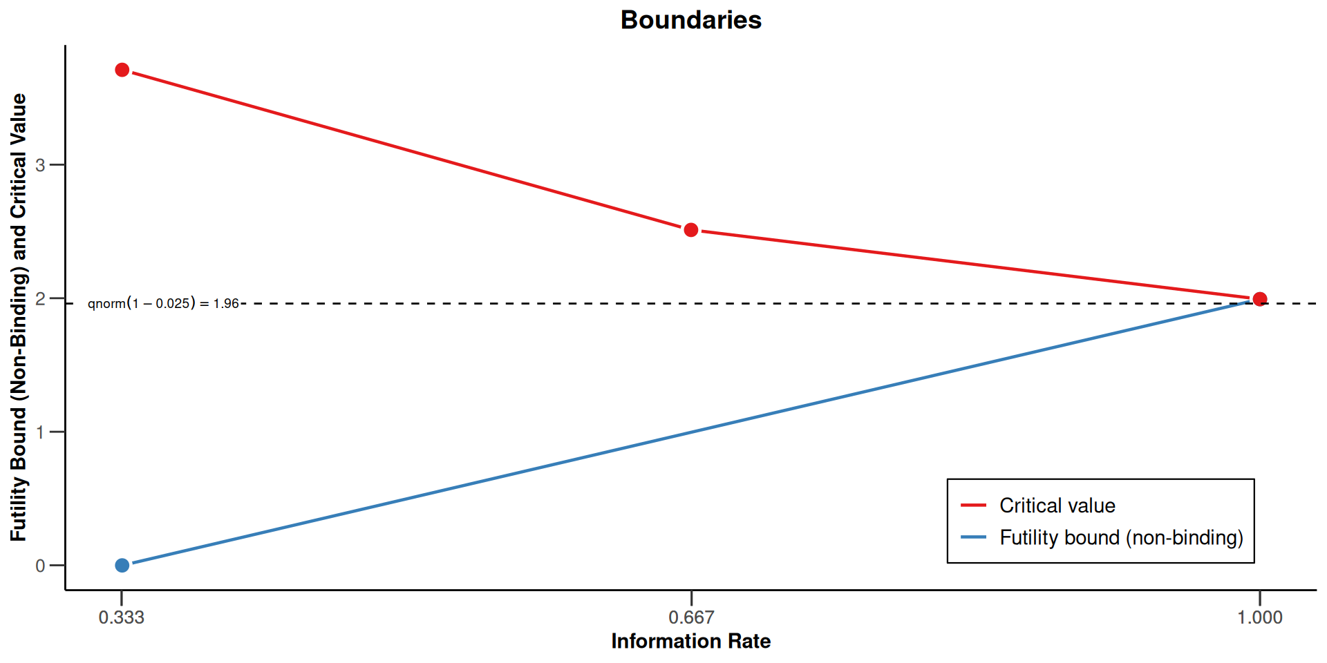
Sequential analysis with a maximum of 3 looks (group sequential design), one-sided overall significance level 2.5%, power 80%. The results were calculated for a two-sample t-test (normal approximation), H0: mu(1) - mu(2) = 0, H1: effect as specified, standard deviation = 1.
Stage
1
2
3
Planned information rate
33.3%
66.7%
100%
Cumulative alpha spent
0.0003
0.0072
0.0250
Stage levels (one-sided)
0.0003
0.0071
0.0225
Efficacy boundary (z-value scale)
3.471
2.454
2.004
Futility boundary (z-value scale)
0
0.500
Efficacy boundary (t), alt. = 0.2
0.416
0.208
0.139
Efficacy boundary (t), alt. = 0.4
0.831
0.416
0.277
Efficacy boundary (t), alt. = 0.6
1.247
0.623
0.416
Efficacy boundary (t), alt. = 0.8
1.663
0.831
0.554
Efficacy boundary (t), alt. = 1
2.078
1.039
0.693
Futility boundary (t), alt. = 0.2
0
0.042
Futility boundary (t), alt. = 0.4
0
0.085
Futility boundary (t), alt. = 0.6
0
0.127
Futility boundary (t), alt. = 0.8
0
0.169
Futility boundary (t), alt. = 1
0
0.212
Cumulative power
0.0359
0.4633
0.8000
Number of subjects, alt. = 0.2
279.0
557.9
836.9
Number of subjects, alt. = 0.4
69.7
139.5
209.2
Number of subjects, alt. = 0.6
31.0
62.0
93.0
Number of subjects, alt. = 0.8
17.4
34.9
52.3
Number of subjects, alt. = 1
11.2
22.3
33.5
Expected number of subjects under H1, alt. = 0.2
666.5
Expected number of subjects under H1, alt. = 0.4
166.6
Expected number of subjects under H1, alt. = 0.6
74.1
Expected number of subjects under H1, alt. = 0.8
41.7
Expected number of subjects under H1, alt. = 1
26.7
Overall exit probability (under H0)
0.5003
0.2459
Overall exit probability (under H1)
0.0833
0.4444
Exit probability for efficacy (under H0)
0.0003
0.0069
Exit probability for efficacy (under H1)
0.0359
0.4274
Exit probability for futility (under H0)
0.5000
0.2391
Exit probability for futility (under H1)
0.0474
0.0171
Legend:
(t): treatment effect scale
alt.: alternative
The function getFutilityBounds()
This new function converts futility bounds between different scales
For one-sided two-stage designs, futility bounds can be specified for different scales which are
the \(z\)-value or \(p\)-value scale
the effect size scale
the reverse conditional power scale
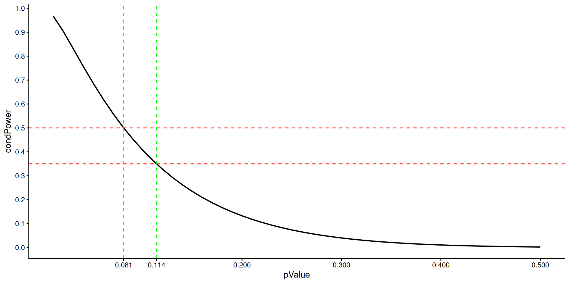
the conditional power scale
Here one can select between:
the conditional power at some specified effect size
the conditional power at observed effect
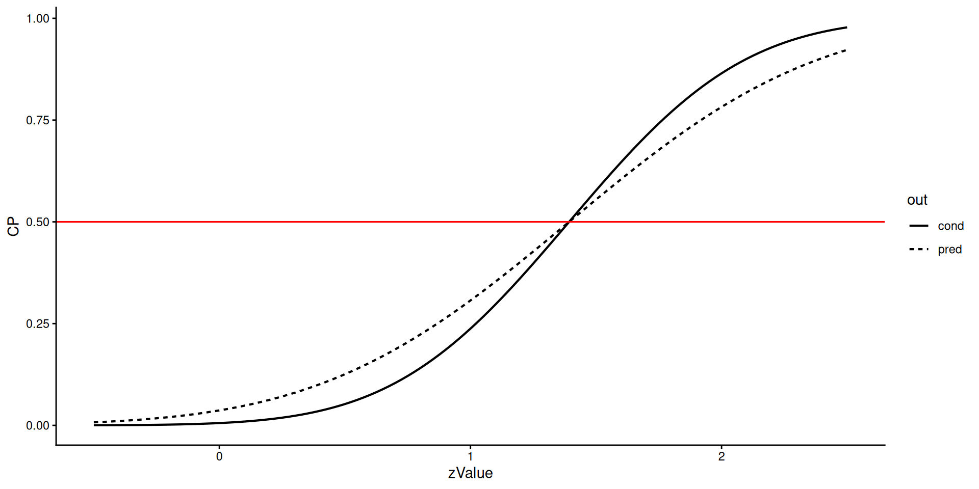
the Bayesian predictive power
This can also be applied to inverse normal or Fisher combination tests
A futility bound \(u_1^0\) on the \(z\,\)-value scale is transformed to the \(p\,\)-value scale and vice versa via \[\begin{equation}
\alpha_0 = 1 - \Phi(u_1^0) \;\hbox{ and }\; u_1^0 = \Phi^{-1}(1 - \alpha_0), \hbox{ respectively}.
\end{equation}\]
Effect size scale
A futility bound \(u_1^0\) on the \(z\,\)-value scale is transformed to the effect size scale and vice versa via
For other testing situations, this needs to be derived accordingly.
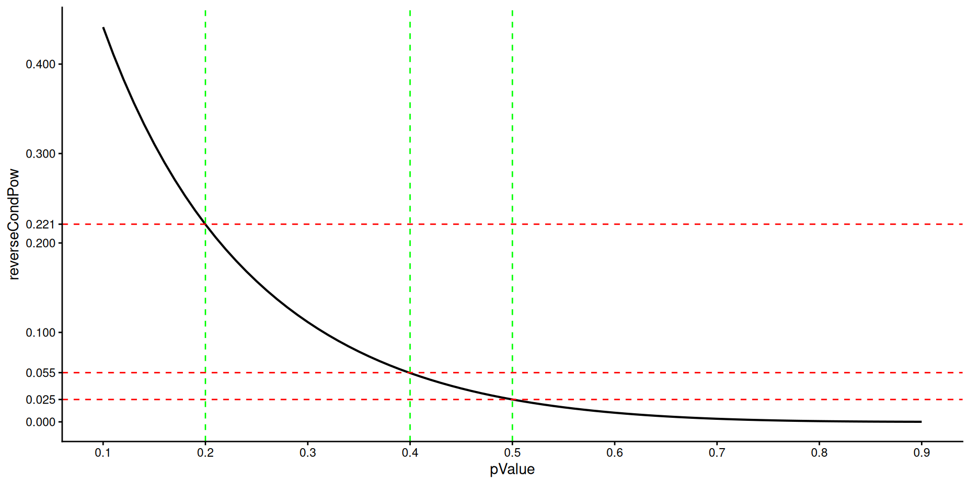
Reverse conditional power scale
According to Tan, Xiong, and Kutner (1998), the reverse conditional power, RCP, is an alternative tool for assessing futility of a trial.
For a two-stage trial using test statistics \(Z_1\) and \(Z_2^*\) at interim and at the final stage, respectively, the RCP is the conditional probability of obtaining results at least as disappointing as the current results given that a significant result will be obtained at the end of the trial.
“Reverse stochastic curtailment”
Let \(t_1\) be the information at interim. The formula for RCP is
which is independent from the alternative because \(Z_2^*\) is a sufficient statistic (cf., Ortega-Villa et al. (2025)).
Notes:
A one-sided two-stage design with rejection boundary for the second stage has to be defined
No need to specify the (absolute) information \(I_1\) at interim, only information rate \(t_1\).
One attractive choice is stopping for futility if RCP \(\leq 0.025\) (\(\widehat = \;\; z \leq 0\) for two-stage design at level \(\alpha = 0.025\) with no early stopping)
Specifying an upper bound \(cp_0\) for the RCP with regard to futility stopping yields
Bayesian predictive power for the group sequential and inverse normal combination case
The Bayesian predictive power using a normal prior \(\pi_0\) with mean \(\delta_0\) and variance \(1 / I_0\) can be shown to be (cf., Wassmer and Brannath (2025), Sect. 7.4)
Promizing zone approach (Mehta and Pocock (2011)): Increase sample size if conditional power at observed effect exceeds 50% (refined values exist). Then traditional test statistic can be used.
Predictive interval plots might be another alternative (cf., Ortega-Villa et al. (2025))
beta spending function might help to construct futility bounds
All boundaries should be considered as guidelines rather than strict rules, i.e., as a non-binding rule.
getFutilityBounds() function as a separate tool
Extensively tested, e.g., through reverse checks
Will be included in sample size and power calculation features, esp., to obtain informations and effect size automatically.
References
Mehta, Cyrus R, and Stuart J Pocock. 2011. “Adaptive Increase in Sample Size When Interim Results Are Promising: A Practical Guide with Examples.”Statistics in Medicine 30 (28): 3267–84.
Ortega-Villa, Ana M, Megan C Grieco, Kevin Rubenstein, Jing Wang, and Michael A Proschan. 2025. “Futility Monitoring in Clinical Trials.”Statistics in Medicine 44 (13-14): e70157.
Tan, Ming, Xiaoping Xiong, and Michael H Kutner. 1998. “Clinical Trial Designs Based on Sequential Conditional Probability Ratio Tests and Reverse Stochastic Curtailing.”Biometrics, 682–95.